Introduction

This is broad overview of Apache Spark, and is designed as a companion piece to my 10,000ft view on Cassandra. The information is derived from the edX course Introduction to Big Data with Apache Spark, from the books Learning Spark and Advanced Analytics with Spark, and from the Spark docs.

What is Spark?

Apache Spark is a general purpose cluster computing engine. Its purpose is to allow us to do work on huge amounts of data very quickly, by taking advantage of modern cluster computing to compute at scale, and by taking advantage of the current low cost of RAM to compute in memory. This makes it much faster than its immediate predecessor, Google’s MapReduce paradigm, which relies on writing to disk during computations. It further improves on the old MapReduce by supporting interactive queries and stream processing, on top of iterative and batch processing. Spark offers APIs in Scala, Java, R and Python (MapReduce only ran in Java), and offers a richer set of possible operations on data.

Like its predecessors, Spark abstracts away the details of distributed computing such as fault tolerance and linear scalability. We just write our programs and Spark works out how many nodes to run them on, and how to recover data from failed nodes. Unlike its predecessors, the overall developer experience with Spark is quite painless. Writing Hadoop programs, for example, is notoriously tortuous. With Spark everything is much easier. And apart from anything else…Scala is awesome as we all know.

Architecture

Spark Components
Spark is made up of several components. There is the core ‘computational engine’ that is responsible for scheduling, distributing, and monitoring applications across many worker machines. Built on top of this core component are several higher-level components that are specialised for certain types of computations. The most notable of these are Spark SQL, Spark Streaming, and MLlib (a machine learning library). These components are all designed to be used together, so you can use them in your Spark programs like you would use normal libraries in your code.

The packaging up of these various components into the one super-tool that we call Spark gives us several benefits. Firstly, whenever an improvement is made to the core component the higher-level components benefit as well. Secondly, the applications that we build using Spark are easier to deploy, maintain and test than if they were built using several independent components. Finally, and most importantly in my opinion, the bundling of components allows us to build applications that use multiple processing models. For example, we can employ a streaming model in our program while also reserving batch processing capabilities for certain situations.

Here are the major components at a glance:

Spark Core – performs the basic functionality of Spark. It schedules tasks, manages memory (which, remember, is Spark’s USP in comparison to other engines), manages fault recovery, and interacts with persistent storage (Spark will write to disk on occasion). Spark Core contains the API for resilient distributed datasets (RDDs), which are Spark’s primary programming abstraction.

Spark SQL – used for working with nice structured data. Supports querying data with SQL, and supports many data formats including JSon.

Spark Streaming – enables us to perform processing on streams of data as they pass through the code. Example data streams are logfiles from web servers or streams of data on web properties that may be produced by some kind of trawler. Spark Streaming includes an API for manipulating streams that is very similar to Spark Core’s RDD API.

MLlib – short for Machine Learning library. Everyone knows that machine learning is big news at the moment due to the Big Data phenomenon. MLlib provides a number of common machine learning algorithms wrapped up in programming primitives. It also provides some programming abstractions over some of the data science tasks that support the use of these algorithms. At the moment MLlib is quite limited in terms of the data analytics that it supports, but with data analytics being to some degree the very raison d’etre for Spark itself, it receives constant attention and upgrades.

While quite different to the above components, the cluster manager (of which there are several varieties) is an important part of Spark. The cluster manager enables Spark’s massive scalability by, well, managing the cluster of Spark nodes. The Standalone Scheduler is the cluster manager that comes out of the box with Spark. Many users choose Apache Mesos or Hadoop Yarn over the Standalone Scheduler.

A Typical Program
A Spark program begins with a dataset. The typical Spark program then performs transformations on the dataset before invoking actions on it. Transformations and actions are described below.

Transformations & Actions
Transformations and actions are the two ways by which we can manipulate RDDs. A transformation allows us to create a new dataset from an existing one. Examples of transformations are filter and map. Say for example we start off with an RDD which contains the list [1, 2, 3, 4]:

ourListRdd = sc.parallelize([1, 2, 3, 4])

sc.parallelize is simply how we are turning our Scala list into an RDD. Let us now apply the filter transformation to the rdd:

ourListRdd.filter(x => x % 2 == 0)

This transformation applies the lamda function in the parentheses to the elements of the RDD and returns a new RDD which contains only the elements for which the function returns true. Therefore we are returned the list [2, 4]. How about we apply a map transformation to this new list (we can chain transformations together):

ourListRDD.filter(x => x % 2 == 0).map(x=> x * 3)

This returns a new, third RDD. What do you think it contains?
Now, a central part of the Spark programming model is that transformations are applied lazily. This means that Spark does not actually compute the various RDDs until an action is called. When an action is called, Spark looks back at the sequence of transformations and then computes them in turn. It will then send the result of the action to the machine in which the driver process is running (remember that transformations are computed in a distributed manner, across the worker nodes), or save the result to disk. What this result is depends on the contents of the RDD that it is derived from, and the particular action that is called. An example should make this clear. The action used here is collect, which returns all of the contents of an RDD as a Scala array to the driver’s machine (other actions may only return the first n elements of an RDD, for example):

firstListRdd = sc.parallelize([1, 2, 3, 4])
secondListRdd = firstListRdd.filter(x => x % 2 == 0)
thirdListRdd = secondListRdd.map(x => x * 3)
thirdListRdd.collect()

So, in this example, neither firstListRdd, secondListRdd or thirdListRdd are ever calculated until collect() is called on thirdListRdd. When collect() is called, Spark looks at the acyclic graph that it has maintained of the transformations and then computes them. The array returned contains the values 6 and 12.
At a high level, all Spark programs follow the same structure. They create RDDs from some input, they derive new RDDs from them using transformations, and perform actions to gather or save data.

The Spark Execution Model
A Spark application consists of a driver process, which is the process that the user is interacting with, and any number of executor processes distributed across the nodes of the cluster. The driver process is in charge of managing the work flow of the running applications (there can be many applications running simultaneously), while the executors are responsible for actually doing the work in the form of tasks.

At the top of Spark’s execution model are jobs. When an action is called within an application a new job is launched to fulfil the action. The job involves Spark looking at its acyclic graph for the sequence of transformations needed by the action and creating an execution plan. The execution plan involves assembling the various transformations into stages, which are run sequentially. Now, each stage corresponds to a collection of tasks, which each run the stage’s code on a different partition of the data. A discrete stage contains a sequence of transformations that can be completed without shuffling the data between nodes in the cluster.

So what determines whether or not the data has to be shuffled? Well, let’s take a look at our example dataset of [1, 2, 3, 4] and the map transformation. We could theoretically split this dataset across four nodes and carry out the map on each subset individually:

[1, 2, 3, 4].map(x => x * 2)

[1].map(x => x * 2) results in [2]
[2].map(x => x * 2) results in [4]
[3].map(x=> x * 2) results in [6]
[4].map(x => x * 2) results in [8]

Each mapping does not require knowledge of any data in any of the other subsets. However, consider the transformation GroupByKey, and an RDD of key/value pairs. If we had split our tuples across partitions we’d have to recombine them:

[(a, 1), (b, 2), (a, 4), (c, 6)].groupByKey() //each tuple is in a different                                                   //partition

(a, 1) results in (a, (1, 4)) when combined with the data in our third partition
(b, 2) results in (b, 2)
(a, 4)
(c, 6) results in (c, 6)

This moving of data across nodes is called shuffling and it is expensive. You want to avoid it as much as possible.

At the end of each stage Spark writes data to disk, which is then read by the next stage.

The acyclic graph that Spark maintains of the transformations in a program allows it to efficiently deal with node failure. The transformations can simply be reapplied to the data on that node according to the graph’s ‘recipe’, thus removing the need for data replication across nodes (as we see with Cassandra, for example). The graph also allows for the partitioning of data in the first place, because as long as each executor has the graph, computations on a dataset can be performed in parallel by splitting up the dataset among the executors.

Running Spark Applications in a Cluster
It’s possible to run Spark in local mode, whereby the driver process and executor processes all run in the same Java process. This is useful for development, but really Spark is interesting when it’s running on a distributed cluster of computers, in distributed mode.

As we hinted at before, Spark employs a master/slave architecture with one driver process coordinating the actions of distributed executor processes. The driver and the executors each run in their own Java process. The driver is where a Spark program’s main() method runs, and it is where the important SparkContext object is created (we will explain the SparkContext later on). It is also where RDDs are created.

The driver has two duties. Firstly it converts the program’s acyclic graph of transformations into an execution plan (which consists of stages, which consist of tasks). The plan’s tasks are sent by the driver to the executors to be computed. Secondly, the driver coordinates the scheduling of individual tasks on executors.

Executors also have two duties. Firstly, they run the tasks sent to them by the driver and return to it the results of the tasks. Secondly, they provide in-memory storage for RDDs that applications instruct them to cache (this is a key feature of Spark programming).

Whenever a Spark application is run in a cluster, the following sequence of events occur:

1. The user submits an application using the spark-submit command or Spark JobServer.
2. spark-submit or Spark JobServer launch the driver program and invokes its main() method.
3. The driver asks the cluster manager to launch executors for it.
4. The cluster manager obliges, and launches executors.
5. The driver runs the application, sending tasks to the executors based on the acyclic graph of the application.
6. Tasks run on the executors to compute and save results.
7. If the driver’s main() method exits or calls SparkContext.stop() the driver will terminate the executors.

Using Spark

Thus far I have taken it for granted that you, dear reader, are using Scala for all your Spark programming needs. But we can also program with Spark in Java, Python and R. So why do we favour Scala? The short answer is that Scala is awesome. However, there are some other powerful arguments for using Scala with Spark that generalise to all use cases. Firstly, Spark itself is written in Scala. This means that your Scala programs are guaranteed to run that bit more seamlessly on the Spark platform than they would if they were written in Python, Java or R. Secondly, since Scala is Spark’s favoured child the Scala versions of the various components/libraries are upgraded before the other versions.

So how do we go about using Spark with Scala? Here I will present an example batch application accompanied by commentary. The example is from the Spark docs:

import org.apache.spark.SparkContext
import org.apache.spark.SparkContext._
import org.apache.spark.SparkConf

object SimpleApp {
def main(args: Array[String]) {
val logFile = “YOUR_SPARK_HOME/README.md”
val conf = new SparkConf().setAppName(“Simple Application”).setMaster(“local”)
val sc = new SparkContext(conf)
val logData = sc.textFile(logFile).cache()
val numAs = logData.filter(line => line.contains(“a”)).count()
val numBs = logData.filter(line => line.contains(“b”)).count()
println(“Lines with a: %s, Lines with b: %s”.format(numAs, numBs))
}
}

So what’s going on in this simple example which is counting the number of occurrences of the letters ‘a’ and ‘b’ in the README file? Inside the main method, we first initialise a simple String object which will be used to create our first RDD later on. Every Spark program must create a SparkContext object which tells Spark how to access the cluster. This SparkContext object needs to be passed a SparkConf which contains information about our particular application. In this example we tell the SparkContext what our application is called, and what URL to use to connect to the cluster. In this case we are telling it to run in local mode.

With a reference to a data source, a SparkContext, and a SparkConf we are now ready to initialise our first RDD (‘logData’). We do by calling textFile() on our SparkContext, and passing it the path to the text file that we want to turn into an RDD. We cache the RDD so that it is saved in memory for when we want to run the application again. This means that when Spark looks at its graph to see what it has to compute, it need not initialise the RDD from the text file a second time. In this way we can save a lot of expensive IO.

Once we have our first RDD we can create new RDDs by applying transformations to it (filter() in this case). Since our program calls the count() action on the RDD that results from applying filter() to logData, Spark computes the RDDs in its graph and returns the final result as a Long to the machine in which the driver process is running. Finally we print the two Long values to the console in the driver’s machine.

Interacting with C*
Spark can talk to Cassandra via DataStax’s Spark Cassandra Connector. We add a dependency to the Connector in our build.sbt file (more on that later), and import the Connector libraries in our application:

import com.datastax.spark.connector._

We can then read from the ‘asset’ table, which is in our ‘assets’ keyspace, like so:

val assetRdd = sc.cassandraTable(“assets”, “asset”)

The above call to Cassandra returns an RDD of key/value pairs, where the key is the column name and the value is a value in the table for that column.

We can write to Cassandra using the saveToCassandra() method that comes with the Spark Cassandra Connector:

assetRdd.saveToCassandra(“assets”, “asset”, AllColumns)

In the above method call we again specify the keyspace and table that we want to save the contents of our RDD to. We also specify the columns in the table that we want to save to. In this case assetRdd has data for every column in the asset table so we don’t need to be specific. We can use ‘AllColumns’. (Note that were we to use the above two calls one after the other in a program, then the call to saveToCassandra would simply be reinserting data that already exists in the table, and the table would not change.)

Deploying Applications in Spark
You have two options if you want to deploy a Spark application:

• spark-submit
• Spark JobServer

spark-submit is the command line program that comes packaged with Spark. It is used to launch an application like so:

spark-submit --class com.gintycorp.stream.sucker.StreamSucker --master spark://colm.gintycorp.com:7077 --deploy-mode client /home/colm/projects/sucker/target/scala-2.10/sucker-assembly-1.2.12.jar local

Regarding the parameters, we are specifying:

• the url of the cluster master to which we are sending the jar and which will distribute the code to its workers
• the deploy mode, which is client in this case. Deploying a Spark application in client mode means that the driver will be external to the actual physical cluster of machines that are running the workers, usually meaning on your local machine. If deployed in cluster mode, the driver will live on a machine in the cluster.
• the jar that we are deploying
• finally, a String parameter which is used by our code to determine the environment in which it’s running (e.g. local, prod, ver)

Spark JobServer is a server that provides a RESTful way to launch Spark applications. We can use it to launch applications from REST services. With the JobServer running in our environment we can upload to it a jar containing our application code, via curl:

curl --data-binary @../../target/scala-2.10/stream-sucker-assembly-1.2.6.jar localhost:8090/jars/interfaceBuilder

We can then kick off a interfaceBuilder job by submitting a request to the REST service.

Spark Web UI
Spark provides a web interface which allows you to track the progress of your jobs, and to query the logs. It is available at 8080 and 4040 by default.

Build.sbt
So how do we build our Spark applications? Well, assuming they are Scala programs, we build them as we do any other Scala program. As mentioned above, there is a file called build.sbt which lives at the root of the Scala project and is roughly equivalent to the root pom of a Maven project. This is the dependencies section of an example build.sbt from Learning Spark:

libraryDependencies ++= Seq(
"org.apache.spark" %% "spark-core" % "1.3.1" % "provided",
"org.apache.spark" %% "spark-sql" % "1.3.1",
"org.apache.spark" %% "spark-hive" % "1.3.1",
"org.apache.spark" %% "spark-streaming" % "1.3.1",
"org.apache.spark" %% "spark-streaming-kafka" % "1.3.1",
"org.apache.spark" %% "spark-streaming-flume" % "1.3.1",
"org.apache.spark" %% "spark-mllib" % "1.3.1",
"org.apache.commons" % "commons-lang3" % "3.0",
"org.eclipse.jetty" % "jetty-client" % "8.1.14.v20131031",
"com.typesafe.play" % "play-json_2.10" % "2.2.1",
"com.fasterxml.jackson.core" % "jackson-databind" % "2.3.3",
"com.fasterxml.jackson.module" % "jackson-module-scala_2.10" % "2.3.3",
"org.elasticsearch" % "elasticsearch-hadoop-mr" % "2.0.0.RC1",
"net.sf.opencsv" % "opencsv" % "2.0",
"com.twitter.elephantbird" % "elephant-bird" % "4.5",
"com.twitter.elephantbird" % "elephant-bird-core" % "4.5",
"com.hadoop.gplcompression" % "hadoop-lzo" % "0.4.17",
"mysql" % "mysql-connector-java" % "5.1.31",
"com.datastax.spark" %% "spark-cassandra-connector" % "1.0.0-rc5",
"com.datastax.spark" %% "spark-cassandra-connector-java" % "1.0.0-rc5",
"com.github.scopt" %% "scopt" % "3.2.0",
"org.scalatest" %% "scalatest" % "2.2.1" % "test",
"com.holdenkarau" %% "spark-testing-base" % "0.0.1" % "test"
)

Libraries

As mentioned above, Spark includes several components which are tightly integrated with Spark Core, and which are interoperable. They can be used together in Spark programs just like third party libraries.

Spark SQL
Spark SQL is Spark’s interface for working with structured and semistructured data. Structured data is any data that has a schema, such as JSon. Spark SQL provides us with DataFrames, which are a programming abstraction designed to simplify the process of working with structured data. A DataFrame is sort of like a table in a relational database.

Spark Streaming
Spark Streaming enables the processing of live data streams from sources such as Twitter, Kafka (a queuing system) and TCP sockets. We can apply the transformations to the stream data, for example filtering the data as it comes in to create a sub-stream of the original stream, just as we create a new smaller RDD by applying filter to an RDD. We can also combine Spark components by applying the algorithms of MLlib to streams of data.

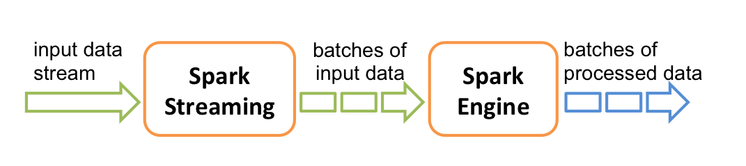
Internally, Spark Streaming works by splitting up incoming data streams into discrete batches. These batches are then fed into a Spark application, which produces a result as a ‘stream’, which is a stream of batches.

Just as Spark Core provides us with RDDs as a high level abstraction over input datasets, Spark Streaming provides us with DStreams. DStreams represent a continuous stream of data, although as mentioned above they are actually a stream of batches of data. In fact, internally DStreams are a sequence of RDDs. Analogous to RDDs, DStreams can be created either from input data streams or by applying transformations to existing DStreams.

Here follows an example Spark Streaming program. It comes from the Spark docs:

import org.apache.spark._
import org.apache.spark.streaming._
import org.apache.spark.streaming.StreamingContext._

Just as we need a SparkContext object for a batch program, we need a StreamingContext object for a streaming program. As well as passing a SparkConf to the StreamingContext we can set the time interval by which to delineate batches of stream data. I.e. we will start a new batch every x seconds.

val conf = new SparkConf().setMaster("local").setAppName("NetworkWordCount")
val ssc = new StreamingContext(conf, Seconds(1))

Using this context we here create a DStream that represents streaming data coming from a TCP source, specified as hostname and port (localhost and 9999 in this case).

val lines = ssc.socketTextStream("localhost", 9999)

This lines DStream represents the stream of data that comes in via the TCP connection. Each record in this DStream is a line of text. Next, we want to split the lines by space characters into words.

val words = lines.flatMap(_.split(" "))

flatmap here splits each line into multiple words and the stream of words is represented as the words DStream. Next, we want to count these words.

val pairs = words.map(word => (word, 1))
val wordCounts = pairs.reduceByKey(_ + _)

wordCounts.print()

The words DStream is mapped to a DStream of (word, 1) pairs, which is then reduced to get the frequency of words in each batch of data. Finally, wordCounts.print() will print the counts that are generated every second.

Note that we have not called an action yet. In this case we are not looking to do anything other than print to the console, and the print() function is not a Spark action. In order to kick off the computation of the transformations we can call the following:

ssc.start()
ssc.awaitTermination()

MLlib
MLlib is Spark’s machine learning library. As mentioned in our Spark Components section, Spark provides abstractions over many common machine learning algorithms and tasks. Not every machine learning algorithm is provided – some algorithms are not suitable for parallel computations over multiple nodes. In these cases Spark can provide no advantage over existing libraries that include these algorithms.

Ultimately, an MLlib program is the same as a Spark Streaming or batch program – it consists of functions called on RDDs. All of the actual data science is hidden under the hood. To use the library effectively, of course, you must have some understanding of data science pipelines (i.e. given a data set and an objective, which tasks and algorithms do I wish to apply). I believe, however, that it is possible to do useful data science using MLlib while only having a rudimentary grasp of data science fundamentals. The two books Data Smart and Data Science for Business contain much of the information that you need.

Conclusion

That is Apache Spark from a high level. In-memory processing and lazy evaluation are the secret sauce, but it pays to have an understanding of the nuts and bolts of the architecture and execution model as well. Hopefully the above will give you that. Also, I hope that I have given you something of a feel of what working with Spark is like, via the examples and the deployment information.

The book Learning Spark has mediocre reviews on Amazon, mostly due to the fact that it is just a repackaging of the information that is already available for free online in the form of the Spark official documentation. However, if you’re like me and you like your technical info neatly organised in book form you will find Learning Spark very valuable. Advanced Analytics in Spark is a book on using Spark for data science, so if you are interested in that give it a look. Finally, the edX course Introduction to Big Data with Apache Spark is informative, and will also help you to exercise your functional chops.

 

 

Introduction

This is essentially a summary of the book, Apache Cassandra Hands-On Training: Level One.

It’s a fairly basic workbook that takes you through Cassandra from a high-level perspective. You can download a VM from the book’s site that gives you a Cassandra instance, and the book walks you through several exercises where you use Cassandra’s most basic functionality.

I found the book very helpful, and it is much smaller than it looks (it really walks you through the exercises in baby steps, and there is quite a lot of material that you can easily skip over – you’ll see what I mean if you take a look through the pages).

 

What is Cassandra?

So, you all probably have a pretty good idea of what Cassandra is, whether you’ve used it in your work or not. It’s an open source NoSQL database that boasts scalability, resiliency, fast reads, and fast writes.

Cassandra allows for linear scalability by distributing your database data across different servers. If you want to scale up, you just scale out, by adding another server. Simples.

Cassandra will continue operating even if some servers go down. This is because the same data can be written to more than one server in a redundant fashion. If a server goes down then another server which hosts the same data can step in and pick up the slack.

Cassandra boasts lightning fast writes. Cassandra reads are far slower than Cassandra writes but are far faster than MySQL reads when dealing with massive amounts of data and large numbers of concurrent users. The details behind Cassandra reads and writes are beyond the scope of this introductory article, but more information can be found here http://www.mikeperham.com/2010/03/17/cassandra-internals-reading/ .

 

Architecture

As mentioned above, with Cassandra your database is spread out across multiple servers. These servers are called nodes, and the nodes together form a cluster. Within a cluster there are no master or slave nodes. Each node is completely equal and has the same functionality as every other node in the cluster. Think of it as like the Hydra, or the Russian Mafia.

There are two abstractions that Cassandra utilises to knit the cluster together: Snitch and Gossip. Snitch is how nodes in a cluster know about the location of each other (IP address, data centre, rack, etc.) Gossip is how nodes in a cluster communicate with each other. Gossip takes place every second, with each node communicating with up to three other nodes, exchanging information about itself and all of the other nodes that it has information about from previous gossip exchanges. While Snitch lets nodes know about the topology of the cluster, Gossip lets nodes know about the state of the nodes in the cluster. For example, is each node up or down.

How does data get distributed in Cassandra? If we have multiple nodes, which data gets sent to which node? Well, for every row of data that is to be written to a Cassandra instance, the row is passed through a hash function (called the partitioner), and then sent to a particular node depending on the hash value that is output by the function. Each node is assigned a range of values when it is added to the cluster, and if a row’s hash value falls within that range then the row goes in that node.

For example, take the following Cassandra table:

 

If we are to assume that home_id is the partition key (the key by which we will assign the row to a node), then each home_id value will be passed into the partitioner and the partitioner will spit out a value between -2⁶³ and 2⁶³. Say, for example, that passing the first home_id H01033638 to the partitioner returns a value of -24887391024765843411. If we have two nodes in our cluster, and Node1 is assigned the range -2⁶³ to 0 while Node2 is assigned the range 1 to 2⁶³, then to which node will the first row of this table be assigned? Answers on a postcard please.

As mentioned previously, resiliency is key to Cassandra’s appeal. Resiliency is achieved by storing data on more than one node. When setting up a database (which we will go into in more detail later), we have the option of specifying a replication factor. If we specify a replication factor of 3 then our row will be written to the node that owns it (determined by the partitioner and token ranges, as discussed above), plus two other nodes in the cluster. If the node that owns the data suffers an unexpected breakdown one of the other two nodes can take ownership of the newly orphaned data. Note that the other two nodes will start off with a range of data which they own, plus the first node’s data which they simply store. If the first node goes down the cluster becomes smaller by one node, and the ranges for the remaining nodes will become larger by some amount.

So, I now have a confession to make. I’ve been lying to you! By default, from Cassandra 2.0 each node is not responsible for one range of hash values. It is responsible for many, by being split up into virtual nodes. The advantage of virtual nodes is that it becomes easier to add a new node to a cluster while maintaining an even distribution of load across all the nodes. In the past, a cluster was expanded by doubling its size, and each existing node had its range simply cut in half. It was considered too difficult to dynamically compute new ranges for each node. Now, by using virtual nodes we can add just one server to the cluster, and it will assume its ‘fair share’ of the load, by taking on some of the virtual nodes that were previously assigned to existing servers. A related advantage of virtual nodes is that is easier to assign different total ranges to different nodes in the cluster. For example, you may want to assign a wider range to a more powerful server and a narrower range to a less powerful one.

 

Using Cassandra

Communicating with Cassandra

To communicate with Cassandra we use its own query language CQL, which is very similar to SQL. We can talk to our cluster via the CQL shell (cqlsh) at the command line, or via a driver program. The former comes in very handy while doing development work.

An example CQL query looks like this. What do you think it is doing?:

 

It is important to note that while CQL is similar to SQL, it lacks some of SQL’s features. This is a weakness of NoSQL databases in general. While they are more scalable and resilient than relational databases, relational databases provide for richer queries.

 

The Structure of a Cassandra Database

A Cassandra database is defined by a keyspace. There may be many keyspaces in a cluster, but each one represents a distinct database. A keyspace can contain tables, in which our data is stored.

When creating a keyspace we need to give Cassandra the desired name for the keyspace, as well as the desired replication factor and the desired class. The class defines whether the cluster can be spread across one or more data centres (the NetworkTopologyStrategy class) or one only (SimpleStrategy). For example, the below keyspace will be stored in a cluster which is spread across two data centres, dc1 and dc2. We can specify replication per datacentre. In this example we have chosen a replication factor of three in dc1 and two in dc2.

 

When messing about with a local Cassandra instance you should set up keyspaces with SimpleStrategy and a replication factor of 1:

 

Creating a Table

In order to create a table Cassandra needs to know which keyspace the table will belong to. We get into a keyspace by using the USE command. E.g.

 

We’re now in the vehicle_tracker keyspace and any table we create will belong to this keyspace. When we create a table we can define the columns of the table. Remember the table that we looked at earlier:

 

We can define this table as follows:

 

We have defined the column names as well as the data types which are allowed in the columns. We have also defined the primary key. As in relational databases, the primary key is a unique value which uniquely identifies each row in a table. In this example, home_id is a unique value and can be used as the primary key. However if home_id was not unique than it could be combined with another value in the row to create a compound primary key:

 

The first column in the primary key will be the partition key, which as I mention in a previous section is the value which the partitioner hashes in order to determine which node to assign the data in the row.

Any columns in the primary key other than the partition key are clustering columns. So, if in our above example home_id is not unique, all rows which have the same value for home_id will find themselves in the same partition. Within this partition rows will then be ordered by the value of the clustering columns.

 

How Data is Stored in Cassandra

When defining our tables in CQL, our data is divided into rows. Internally in Cassandra, however, the data is not stored in rows. Rather, it is stored in partitions. Take the following table, which has the primary key ‘(home_id, datetime)’:

 

While this table has three rows, since each row has the same partition key (the first column of the primary key) the data is stored in a single partition within Cassandra:

 

You can see that the data in the partition is ordered by the datetime value, since datetime is the clustering column.

 

How Data is Stored on Disk

When we write data to a table in Cassandra, it is stored to a commit log on disk and to memory. The data in memory is called memcache. When the memcache for a particular table is full it is flushed to disk as an SSTable. The SSTable can be thought of as a snapshot of a table, containing a relatively up to date version of its data. The data in the SSTable can change as you edit the table via CQL commands. The commit log on the other hand, is a record of all commands which is kept so that the commands can be reissued sequentially if a node ever goes down and has to be brought back up from scratch.

 

Modelling Data

Before we build a data model it is important to understand the limitations of NoSQL distributed databases compared to relational databases. The most important limitation is that SQL joins are not possible. Since the data you are joining may be spread across several different machines, joins would be extremely slow. Therefore, you must think in advance of the queries that you expect to be making, and model your data so that all the data for any one query is contained in a single table. While the data in a single table may be spread across multiple machines, its data is indexed, which is all-important.

This leads us to a further limitation which is that WHERE clauses in Cassandra should reference a partition key. This is because our data is indexed by partition key, and since the data is distributed it would be extremely inefficient to reference data that isn’t indexed. For example, using the previous table which has the primary key (home_id, datetime), the following query would work:

 

This query would also work, since we can reference the clustering column if we also reference the partition key:

 

This query, however, would blow up since we are referencing a column that isn’t part of the primary key (even though we are still referencing the partition key):

 

There is an exception to the above point re: WHERE clauses only referencing values in the primary key. By creating a secondary index on a non-primary key column, we can reference values in columns other than the primary key. However, querying using secondary indexes is slow – the query has to examine a special secondary indexes table on every node in the cluster.

A final thing to consider about modelling data in Cassandra is this: what if a partition can grow infinitely? For example, imagine a table that stores data about a vehicle and its GPS coordinates at a particular point in time:

 

Say the above table’s partition key is the vehicle_id. We could potentially track the coordinates of one vehicle for a very long time. In that case the partition storing rows for that vehicle_id could grow extremely large. There is a limit to the number of rows that can be stored in a partition in Cassandra, and there is a limit to the amount of data that can fit on disk on one node (all data for a partition must live on one node). While these numbers are very large, they are finite. Therefore it is wise to guard against partitions that have the potential to become extremely large by using composite partition keys. For example, the partition key for the above table could be vehicle_id and date. The values in the two columns are combined and fed into the partitioner.

 

Conclusion

This concludes our high level overview of Cassandra. If you are interested to learn more, I would recommend that you dive into the book that this article is derived from. It contains many exercises that you can work through, which will give you hands-on experience with issuing CQL commands and manipulating Cassandra databases. The book also contains recommendations for other resources that you can use to continue your education in all things Cassandra.

Introduction

In my previous post I explained how data science has been used by organisations to gain competitive advantage. In this post I will explain how I see the company I work for, a fairly typical modern software company, gaining competitive advantage from data science. Like the last post this is an adaptation of a posting that I shared internally with my colleagues.

Sales

Where I work we do ‘digital governance’. The major part of our value proposition is a platform which monitors the quality of clients’ websites and allows them to easily manage what are usually (in our clients’ cases) massive, sprawling things.

Every day there are 500 million tweets sent. Some non-trivial portion of those tweets are related to issues of website quality and governance. It is possible to perform something called sentiment analysis on these tweets to determine the attitude of the tweeter towards those issues. Are they frustrated with their current governance framework? Are they frustrated by the lack of any framework at all? If we could narrow down the set of all tweets to those that would be promising sales prospects for us, then that would be a valuable thing. And we can do that, using the aforementioned sentiment analysis along with textual data analysis.

Improved system uptime

Despite the best efforts of our dev team and especially our ops team, our systems break down sometimes, affecting the end user’s experience. This is bad. Fortunately, there exist techniques called predictive modelling and cluster analysis which can help us to predict and avoid future breakdowns. Essentially, we can collect the system data from around the time of the problem and feed it into a model which will look for, and hopefully find, patterns. These patterns can help us diagnose the root cause of problems, as well as give us advance warnings of when they are about to happen again.

Business problem optimisation

The set of techniques called optimisation involves translating a real-world business problem into its mathematical formulation, and then solving the mathematical representation for the best solution. This is an application of data science that far predates the current hype around the field. It has applications for all types of business problems, e.g. managing workforce churn, purchasing, and cash management.

Pleasant surprises

As I mentioned at the end of my previous post, data science can give us insights that we were not specifically looking for. There are a group of techniques which involve feeding a data set into a model, running the model, and seeing what insights the model throws up. These techniques are collectively called unsupervised data mining, and they can throw up insights such as clusters of similar objects, outliers, local influencers among groups, and bridges between different groups. I think it is obvious how such insights might help our sales efforts, for example.

Other opportunities

I hope that the opportunities that I have outlined above seem interesting at the very least. I am not an expert on data science, and it is certain that with more knowledge I could find more and more opportunities in the business I work in for the profitable application of data science. Were others in the business to acquire only some data science knowledge, new ideas would start sprouting from all directions. This leads me to my next point…

Develop in-house capabilities

Data science capability is rare. There just aren’t that many qualified data scientists out there. This will change in the next 5-10 years as universities adapt to market forces, but right now it is difficult for a firm to acquire external data science capability. Any firm that does acquire data science capability will therefore have a large competitive advantage. In my company we don’t have data scientists, but we do have many skilled software developers of an analytic bent. It is very feasible that they can quickly learn the more basic of the techniques that I mentioned in earlier paragraphs. All tech companies are the same.

Look outside?

While it is very difficult and expensive, currently, to bring in a data scientist as a permanent member of staff, there are ways that an organisation can acquire capability without developing it internally, and without breaking the bank. These are all practices recommended in the book Data Science for Business:

• Fund academic research. PhD students work for peanuts, and if an organisation can exploit them encourage them to work on its problems, it can get them solved very cheaply. Of course, the results will be shared with the academic community and therefore may be available to competitors.
• Take on a data scientist as a ‘scientific advisor’.
• Hire a third party firm to do your data science. The book notes the caveat that the interests of data science firms are not always well aligned with the interests of their customers. The authors don’t go into detail on what they mean by that.
• Post a competition on Kaggle.com, a site which allows organisations to post problems along with a prize. The competitions are open to the public, and often attract excellent data scientists. NASA has used the site in the past to gather solutions to its data science problems.

Now for the threats…

The flip side of everything that I’ve said in this post is that our competitors may profitably do data science, and may use it to gain a competitive advantage over us. We should be aware of this threat. What data do our competitors collect that we don’t, and how may it be used by them to gain a competitive advantage? What data science capability do they have that we don’t? Is there a way that a purely data-driven firm may enter our field and do through data what we do through consultancy, thereby eroding one of our key competitive advantages?

Data science is an equal opportunities tool 🙂

 
The following post is adapted from something that I shared in my workplace. We are a medium-sized SME that provides a ‘data-analysis’ service to our customers around issues of website quality and digital governance. We don’t do ‘proper data science’. The document that I wrote up and shared around contained my thoughts on how we could profitably begin doing data science, based on my rudimentary knowledge of the field.
 

What is data science?

Data science is, to quote the author and data scientist John Foreman, “The transformation of data using mathematics and statistics into valuable insights, decisions and products.”

Simples 

Today the hot topic in data science is Big Data, and the two terms are often conflated. However, Big Data is a subset of data science. While a precise definition of Big Data is hard to come by, I believe it is safe to think of it as the application of data science techniques to complete data sets. Until about ten years ago, due to technological constraints, it was impossible to deal with complete data sets, and data scientists used random sampling to garner representative sets of a manageable size from the entire data set.
 
 

Why I have chosen to blog about this?

We don’t do data science in my workplace, so why did I choose to write about it? I wanted to write a blog post, and in terms of things that are directly relevant to our work, I didn’t feel there was much that I could write about that others in our dev function didn’t already know. I’m still only a junior developer 😦 Data science is something that I find very interesting personally, and I spend a bit of my spare time learning about it. We are moving to a new architecture that has a bit of a ‘Big Data’ flavour to it, and as we grow our client-base we are managing more and more data. Therefore I thought an introduction to data science may be of interest to my colleagues.

 

Data science that we’re currently doing

We currently do a lot of data analysis – as in we take in data about our clients’ web estates and run it through our proprietary analysis engine. It could be fairly argued that we are doing Big Data, since we use more or less all of our clients’ data as opposed to a small sample of it. However we are not doing data science as it is generally understood. We are not using techniques such as regression or clustering, for example, to derive insight from the data. We are merely analysing and commenting on the quality of the client’s web estate.

Now, we are not a data science company, and our clients do not pay us to provide them with insight gathered from the website data. However, I argued that we can gain internal value from doing data science that will help us to both serve our customers better and to run a tighter and more efficient ship.

 

Broader data science environment and opportunities

Big data and data science are big news at the moment, and have been for a while. How did this interest come about? Essentially, computing power and storage have become cheap, giving even small organisations the ability to store and access enormous data sets. This new access to such data sets led to the creation of new open-source technologies which are themselves hot topics in the tech community.

Many firms have used this new frontier in data science (enabled by cheap computing and storage) to gain competitive advantage. Amazon are probably the best known, having found ways to use their vast troves of data to provide their customers with targeted product recommendations based on the customers’ past purchases, as well as the customers’ similarity to other customers in Amazon’s data stores. However, as mentioned above, it is not only large organisations that can take advantage of the new frontier. Firms of all sizes, in all sorts of industries are profiting. This has been proven through empirical research, with MIT being just one institution that have evaluated the performance of data-driven companies against others. They have found conclusively that these companies perform better than their competitors, and this result holds for all sizes of companies across all industries. In short, data science is good news, and today there are more opportunities in data science than ever before.

You may be wondering, do all firms have enough data to make an investment in data science worthwhile? Perhaps there is a certain threshold of ‘data-wealth’ that a firm must lie above? Well, certainly it is true that you must have data in order to do data science. However, we are all more data rich than we probably realise (speaking of both organisations and individuals). There are many, many open APIs out there. Private firms such as Google and Twitter have made much of their data open and free to the rest of the world. Similarly, the US government has made vast amounts of its data open to the world. The UK government has followed suit. Theoretically (and realistically!), an organisation could profitably employ data science without any data of its own.

However, at my company we do have data, and lots of it. We have the data that we pull from our clients’ web properties, and we have data generated by our own systems. This data is tiny compared to the data held by the Twitters, Facebooks and Googles of this world, but it is significant. And this data may be more valuable than it seems at first. Information generated for one purpose can be reused for another purpose. Old datasets that seem obsolete on the surface can be merged with other datasets, old or new, to create new value.

 

What exactly can data science do for us?

In my next post I will explain some specific data science opportunities that I see for my company. For now, I will try to outline in broad terms what the field can bring to an organisation. Simply put, it can help us to solve business problems. Think of any of the problems and challenges that the average company faces. How can they make more sales? How can they retain more of their customers? How can they convince new and existing customers to pay more for their service? How can they have less system downtime? How can they provide a faster service to their customers? All of these problems, and many more, can be expressed as data science problems.

But that’s not all! Data science can also provide us valuable answers to questions that we didn’t even ask, and might never have thought to ask. Cool eh?

Introduction

In this blog post I will do my best to explain a selection of Scala concepts. The original motivation behind the post was to improve my own understanding, since it’s a truism that the best way to learn is to teach. The concepts were chosen because they are in some way fundamental to using Scala and because I wasn’t happy with my level of understanding. Most of the concepts are Scala functions, but I’ve thrown in discussions of the underscore, and of currying. Hopefully the following will prove at least a little useful to those that have taken the Functional Programming Principles in Scala course on Coursera, and to those that have yet to take the course. (If you haven’t taken it yet, you should. It’s great)

 

map

map is perhaps the most important tool that a functional programmer has. Essentially, given a collection, we apply a function to every member and return a new collection containing the results of applying that function to the members. So for example, take

We may, for some reason, wish to obtain a new list which contains each element of this list, incremented by one. In other words, we want to apply the following function to each element:

x => x + 1 (for each element, represented by ‘x’, we return an element which is x + 1)

With map this is easy:

This returns a new List, List(1002, 6, 15, 2, 100).

 

flatMap

flatMap is similar to map, except that it can only be given functions that return a sequence. Ultimately you will then have a sequence of sequences which can then be ‘flattened’ into one long sequence. Confused? Good.

Take the previous example. list.flatMap(x => x + 1) would throw an error because the function returns an int, and a sequence of ints (like List(1002, 6, 15, 2, 100) cannot be flattened any further. However, list.flatMap(x => List(x, x + 1)) would work because that function returns a List. We end up with a List of Lists (List(List(1001, 1002), List(5, 6), List(14, 15), List(1, 2), List(99, 100)), which can then be flattened. The result of the flattening is List(1001, 1002, 5, 6, 14, 15, 1, 2, 99, 100).

So, given our example of list.flatMap(x => List(x, x + 1)), this is what happens:

1)      First a map is performed which takes each element and returns a List of the element and the element plus 1. The result of the map function is a List of these Lists.

2)      A flattening is performed which turns the List of Lists into one single List. (There is a Scala method ‘flatten’. flatMap is equivalent to performing a map followed by a flatten).

 

filter

Another important Scala function is filter. filter iterates over a sequence and tests each element against a Boolean expression. A new sequence is returned which contains all elements for which the expression returned true. Here is an example, using the same list that we have used for previous examples:

This returns List(1001, 14, 99).

 

Underscore

This may be a good time to take a break from explaining functions to explaining the underscore character and how it is used in Scala. It has several different uses, but the average reader will probably use it most often in anonymous functions (functions that are used without assigning them to a variable name, as with x => x > 10 in the filter example). _ essentially is used to represent ‘the generic element’ that is the subject of the function. Its usage is probably best understood by example, so I will rewrite two of the anonymous functions that we’ve seen before using the underscore:

 

The underscore can also simply be used as a placeholder in function parameters, instead of the usual ‘x’. See the groupBy examples below. If you replace the underscores with an ‘x’ you should be able to understand what the function is doing.

 

groupBy

groupBy allows us to, you guessed it, group elements of a collection together according to some characteristic. It returns a map of key value pairs where the key is the grouping characteristic and the values are the elements of the collection. Here are some examples:

 

 

 

reduceLeft & reduceRight

These two operations iterate through a sequence, applying a function to each element in turn with respect to an accumulator. That doesn’t help you? I don’t blame you. Here’s a few examples that will hopefully make things more clear:

 

 

The result of calling the above function is 1120, the sum of all the elements in the list. We have passed an operation (_ +_) to reduceLeft, which has the effect of iterating through the list from left to right, adding the right-hand operand to the result of the previous operation. So, in our example we first add 1001 to 5 to give us 1006. Moving down the list by one place, we have 14 as the right-hand operand. We add it to the result of our previous operation, 1006, to give us 1020. We move down one place so that 1 is our right-hand operand and we add it to 1020. Finally we add 99 to our previous result.

Calling list.reduceRight(_ + _) would yield the same result, as the function iterates through the list from right to left. However, list.reduceLeft(_ – _) and list.reduceRight(_ – _) WILL NOT yield the same result. reduceLeft is equivalent to 1001 – 5 – 14 – 1 – 99 = 882. reduceRight is equivalent to 1001 – (5 – (14 – (1 – 99))) = 1008.

Here are some more operations on our list using reduceLeft and reduceRight. Try them out in a scala worksheet to see if the result tallies with your understanding:

 

 

 

foldLeft & foldRight

These two functions are broadly similar to reduceLeft and reduceRight, but they work slightly differently. Here we apply them to our list:

 

 

These two examples both evaluate to the sum of the elements of the list. We are passing an extra parameter to the function (‘0’ in this case), which is our ‘start’ value. Whereas reduceLeft and reduceRight iterated over the list beginning with the first or last two elements, foldLeft and foldRight begin with this ‘start’ value and the first or last element. So the value you give this extra parameter affects the result that you are returned. If you wanted to find the product of the elements, you would choose ‘1’ as the start value. Do you see why?

Again, the subtraction operation yields unexpected results:

list.foldLeft(0)((x, y) => x – y) yields 0 – 1001 – 5 – 14 – 1 – 99, while list.foldRight(0)((x, y) => x – y) yields 1001 – (5 – (14 – (1 – (99 – 0). However, list.foldRight(0)((x, y) => y – x) yields 0 – 99 – 1 – 14 – 5 – 1001.

 

Currying

Currying probably isn’t all that important for a Scala beginner, but I’ve had trouble getting my head around it, conceptually, so I want to outline it here so as to make sure that I understand it. Essentially, currying means that we break down a function that takes multiple arguments into a chain of functions that each take a single argument, and return a function which also takes a single argument, until the last function is called which returns the answer. I will present a function taking multiple arguments and its curried equivalent(s). Hopefully that will illustrate the concept.

Uncurried

 

Curried

 

Alternatively, equivalent(1)(5)(11) also returns 17, as does first(5)(11).

Introduction

This blog post, my first, will be a slightly unusual one, drawing as it does from my undergraduate thesis (I studied Philosophy). I will talk about a concept called the Typical Mind Fallacy, and how it can be applied to the field of information technology.You won’t learn anything technical. Ideally though, after reading this post you will feel ready to adopt a more even, accepting and ‘zen’ attitude towards the behaviour of other people that you come across in the course of your work. I’ll start with a lengthy explanation of the fallacy, because I think you’ll find it interesting, and then I’ll describe just a few of the ways in which the fallacy may come into our daily lives as developers/ops…ers/CTOs/etc.

The Typical Mind Fallacy

The typical mind fallacy is a term coined by an old professor of mine (David Berman) to describe the mistaken belief that all minds are the same, and that there is uniformity to the way that people think and perceive the world around them. The concept was previously described by Arthur Danto, an American philosopher who you probably won’t have heard of, and William James, the famous American psychologist. Those two, like my professor and I, believed that all people naturally tend towards the fallacy, and it is only experience and education that allows us to see that others may have radically different perspectives than our own.

It’s likely that the first time that it was demonstrated that there are significant differences in how we think was in the late 19^th century. Francis Galton, an English scientist, presented a questionnaire to a number of people, asking them to describe their breakfast table in as much detail as possible. His aim was to discover how mental imaging ability was distributed among the population. He discovered a bell curve of imaging ability, with most people in the middle, describing their breakfast table in moderate detail, and a few at either end. Of those at the end, some could describe their breakfast table in ‘photographic’ detail, and a similar number had no imaging ability at all. These people were only able to discuss abstract concepts, and could not ‘see’ the scene of their table in their mind’s eye. Before Galton, it was believed that imaging ability was fairly evenly distributed amongst the population and that while it may differ somewhat in degree it did not differ in kind. However, Galton’s results showed that not only was the range of imaging ability enormous, but also that there were several types of imagers. There were non-imagers, eidetic (or ‘photographic’) imagers, and synaesthetic imagers. Synaesthesia is a fascinating condition whereby ‘stimulation of one sensory modality automatically triggers a perception in a second modality, in the absence of direct stimulation to this second modality’. For example, a sound may trigger a visual perception of colour, even though no colour has been seen by the eyes. For Vladimir Nabokov, the author of Lolita, reading the letters of the alphabet would invoke a particular synaesthetic colour perception. He even had a private word for ‘rainbow’: kzspygv. Each letter corresponds to a colour in the spectrum of light.

Back to Galton. He found that men of science typically had little mental imagery, and moreover, they tended to insist that anybody who claimed to have mental imagery was either confused or lying. James wrote how his subjects with strong imagery found it hard to understand how anybody without this power managed to think at all! So, this is the essence of the typical mind fallacy. We can only possibly be aware of our own mental processes, and therefore we naturally have difficulty imagining processes that are very different from our own. It takes considerable effort to stop ourselves from constantly projecting our own thinking onto others.

How It Affects Us

Perhaps you can now see how easily the fallacy comes in to play, especially in our interpersonal communications. As a weak imager myself, I’ve lost count of the number of times that people have asked me to visualize something, to be amazed when I tell them that I can’t do it. Ask me to visualize a database schema and you’ll be met with a blank look, but ask me to understand the abstract interactions between different modules in a system and you’ll be ‘talking my language’.

So far, the examples of differing minds that we’ve looked at have involved innate differences between minds. The hardwiring, so to speak. We haven’t even mentioned differences in age, gender, place of birth, life experience, position in an organizational hierarchy, etc, etc. All of these factors can cause perspectives on the world to diverge.

Have you ever seen somebody make a technology choice that just seemed absolutely inexplicable? Perhaps you were working in a large organisation and a manager chose technology that was undeniably the wrong choice for the business? Perhaps you cursed the manager under your breath and were bitter about it for days? Unless the manager was a complete idiot (which of course is possible), what happened was that while you were driven purely by the needs of the business, the manager had other motivations that conflicted with the business’ needs. For example, higher managers in large organisations often have to deal with a lot of politics, and these politics can put pressure on technology choices. In this hypothetical case you (hypothetically speaking) probably assumed that the manager was also primarily driven by the needs of the business. Why then did he choose an inferior technology? Is he an idiot? No, he was simply looking at the world through a slightly different lens than you.

Another case that perfectly illustrates the fallacy is the difficulty of intercultural communication. In some East Asian cultures, for example, it is considered impolite to disagree with somebody. Therefore a person that has grown up in this culture will often agree to a request, and then quietly go off and, well, not do it. Many Western people are aware of this cultural difference. But do you remember your interactions with people from these cultures, before you were educated on the difference? Perhaps you found it infuriating? However, the other person is looking through a different lens that is probably equally as valid as yours.

In the SME at which I work, off the top of my head, we have the following differing perspectives:

• The broad, holistic perspective of CTO, Product Owner, Scrum Master versus the narrower focus of a developer.
• Junior developers who are focused on learning versus senior developers who are more focused on getting the job done.
• By my count, in the dev function alone, we have 6 different nationalities, from three different continents.
• Ages ranging from early thirties to whatever age my manager is.

Therefore…

Therefore, although my colleagues and I all have a huge amount in common, it is absolutely certain that we each will bring a completely unique perspective to many aspects of our work. It’s perhaps a little counter-intuitive, but by recognising our differences we can be more understanding and empathetic people, and have a happier and less stressful work life. I would encourage you to consider what I have written here, and to reflect on whether you can profitably adjust your own interactions with, and reactions to, your own colleagues.